C++: a simple geomagnetic field model

A simple geomagnetic field model (including contributions from the Earth's dipole, the effective mirror dipole and the cross-tail current) based on (with minor modifications) [1], [2].

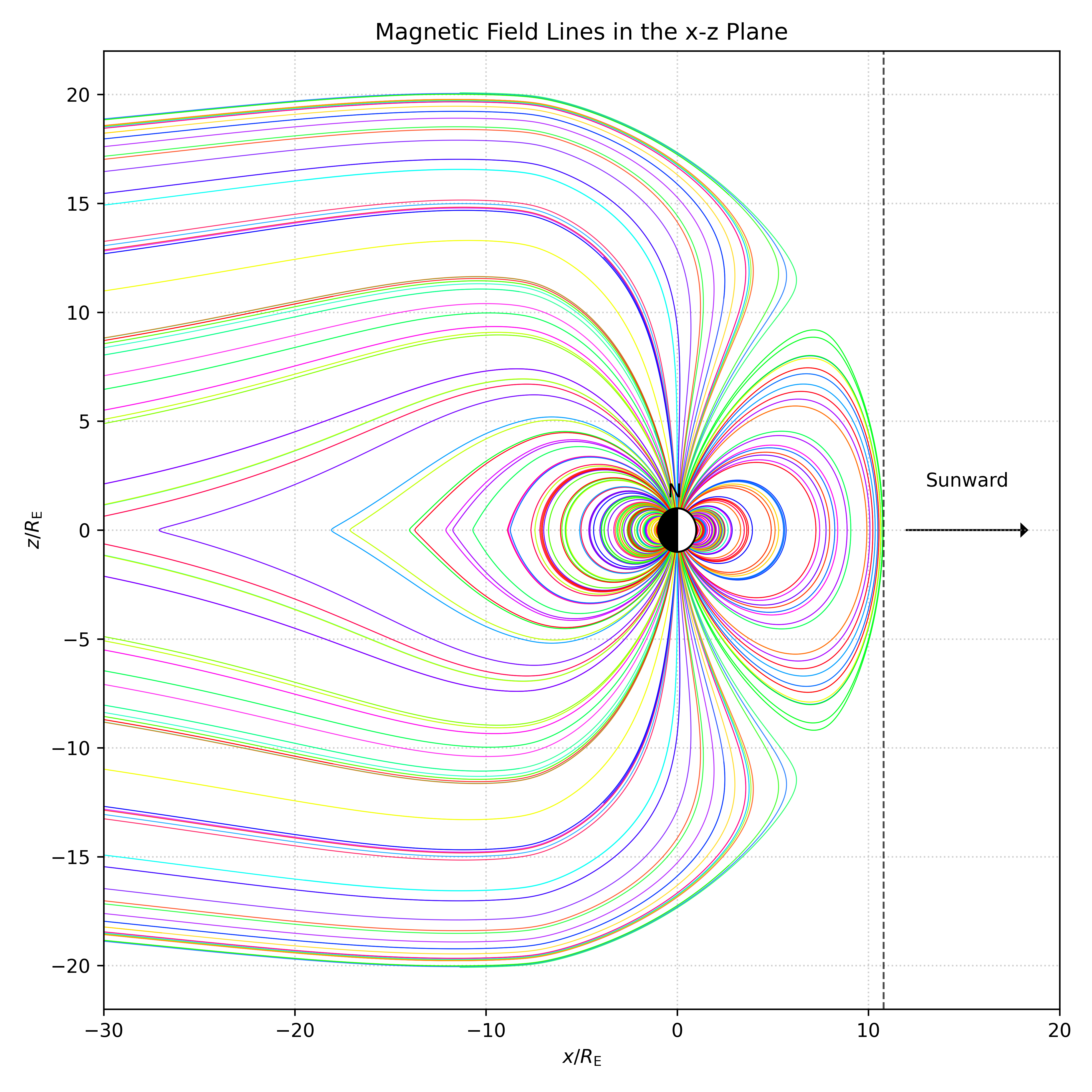Plot of the magnetic field lines in the magnetosphere.

// gmf_th65.hpp
#if !defined(GMF_TH65_HPP)
#define GMF_TH65_HPP

#include <algorithm>
#include <array>
#include <cmath>
#include <cstddef>
#include <numeric>
#include <ranges>
#include <span>

namespace gmf_th65 { // "gmf" for "geomagnetic field", "th65" for "Taylor and Hones, 1965"

    // 给 std::array 定义矢量加法和归一化；其他一些方便运算也可以定义，但这里用不上
    namespace {
        template <typename T, std::size_t N>
        std::array<T, N> operator+(const std::array<T, N>& lhs, const std::array<T, N>& rhs)
        {
            std::array<T, N> result;
            std::ranges::transform(lhs, rhs, result.begin(), std::plus<T>()); // 性能似乎不如手写循环，make sure you measure it!
            return result;
        }
        template <typename T, std::size_t N>
        void normalize(std::array<T, N>& v)
        {
            // 平方和 ⇔ 自身内积
            T norm_v = std::sqrt(std::inner_product(v.cbegin(), v.cend(), v.cbegin(), static_cast<T>(0)));
            // 逐元素归一化
            std::ranges::transform(v, v.begin(), [norm_v](T x) { return x / norm_v; });
        }
    }

    // 地球的偶极场
    std::array<double, 3> earth_dipole_magnetic_field(double x, double y, double z, double correction_factor = 1.0)
    {
        constexpr double B0 { 3.11e4 }; // dipole 的磁场强度，单位为 nT * RE^3
        double r2 { x * x + y * y + z * z };

        // if (r2 < 1.0) return { 0.0, 0.0, 0.0 }; // 如果在地球内部，磁场强度为零

        double factor { correction_factor * B0 / (r2 * r2 * std::sqrt(r2)) };
        std::array<double, 3> magnetic_field;
        magnetic_field[0] = -3.0 * x * z * factor;
        magnetic_field[1] = -3.0 * y * z * factor;
        magnetic_field[2] = -(2.0 * z * z - x * x - y * y) * factor;

        return magnetic_field;
    }

    // 越尾电流片的磁场
    std::array<double, 3> cross_tail_current_magnetic_field(double x, double y, double z)
    {
        // 电流片在 y 方向上的尺度
        constexpr double width { 20.0 };
        double y_profile { std::exp(-(y * y) / (width * width)) };

        // 电流片在 x 方向上的尺度, 以 RE 为单位
        constexpr double sstart { -6.0 }; // 电流开始出现的位置，这里取为偶极场描述开始出现较大误差处
        constexpr double start { -10.0 }; // 电流片强度刚达到饱和的位置，参考《磁层物理》
        constexpr double end { -40.0 }; // 电流片强度开始衰减的位置，参考《磁层物理》
        constexpr double endd { -200.0 }; // 电流片完全消失的位置，参考《磁层物理》

        double tf { std::tanh((x * 4.0 - 2.0 * (start + sstart)) / (start - sstart)) };
        double tg { std::tanh((x * 4.0 - 2.0 * (end + endd)) / (end - endd)) };

        double f { 0.5 * (1.0 + tf) };
        double g { 0.5 * (1.0 + tg) };

        double x_profile { f * g }; // x 方向电流缓变

        // ---------- Bz 如此这般地选取，使得磁场散度为零 ----------
        // double df_dx { 4.0 / (start - sstart) * (1.0 - tf * tf) };
        // double dg_dx { 4.0 / (end - endd) * (1.0 - tg * tg) };

        // double dX_dx { df_dx * g + f * dg_dx };

        // 电流片在 z 方向上的尺度
        constexpr double half_thick { 0.16 / 2.0 }; // 电流片厚度（约 1000 km，参考《磁层物理》）的一半；Taylor and Hones, 1965 取电流片厚度为 0.5
        // 稳定计算 ln(cosh(z/L))
        double u { z / half_thick };
        // double log_cosh_u {};
        // if (std::abs(u) > 20.0)
        //     log_cosh_u = std::abs(u) - std::log(2.0);  // 避免溢出
        // else
        //     log_cosh_u = std::log(std::cosh(u));

        constexpr double B0 { 25.0 }; // nT，参考《磁层物理》；Taylor and Hones, 1965 取 30 nT, 并且声称这个值影响不大

        double Bx { B0 * x_profile * y_profile * std::tanh(u) };

        // double Bz { -B0 * half_thick * log_cosh_u * y_profile * dX_dx };

        return std::array<double, 3> { Bx, 0.0, 0.0 }; // { Bx, 0.0, Bz }; // 磁场散度为零
    }

    // 总磁场，tpye = void (*)(RealType, std::span<const RealType>, std::span<RealType>) 适合 rk4 调用
    void magnetic_field(double /* t unused */, std::span<const double> position, std::span<double> dydx)
    {
        double x { position[0] };
        double y { position[1] };
        double z { position[2] };

        constexpr double mirror_dipole_distance { 40.0 }; // dipole 跟地心的间距，以 RE 为单位
        constexpr double mirror_dipole_strength_ratio { 28.0 }; // dipole 的磁矩与地球磁矩的比值

        std::array<double, 3> tot_field { earth_dipole_magnetic_field(x, y, z)
                                    + earth_dipole_magnetic_field(x - mirror_dipole_distance, y, z, mirror_dipole_strength_ratio) // 等效源，并非严格的镜像
                                    + cross_tail_current_magnetic_field(x, y, z) };
        normalize(tot_field);
        dydx[0] = tot_field[0];
        dydx[1] = tot_field[1];
        dydx[2] = tot_field[2];
    }
}

#endif // GMF_TH65_HPP

Bibliography

- [1] H. E. Taylor and E. W. Hones Jr., “Adiabatic motion of auroral particles in a model of the electric and magnetic fields surrounding the Earth,” Journal of Geophysical Research (1896-1977), vol. 70, no. 15, pp. 3605–3628, 1965, doi: https://doi.org/10.1029/JZ070i015p03605.
- [2] 涂传冶,宗秋刚,周煦之, 日地空间物理学(下册)磁层物理, 2nd ed. 科学出版社, 2020.